Chapter 8: Discrete Probability
Chance, conditioning, Bayes' theorem and expectation
Learning outcomes
After this chapter you should be able to:
- describe a random experiment by its sample space, events and a probability distribution, and compute probabilities by counting when outcomes are equally likely;
- use the rules for complements and unions, and solve problems such as the birthday problem;
- compute conditional probabilities, draw and use tree diagrams, and decide whether events are independent;
- apply Bayes' theorem, and explain why a positive result from an accurate test can still be unlikely to be right;
- work with random variables, the binomial and geometric distributions, expectation and variance, and use linearity of expectation with indicator variables.
8.1 Sample spaces and events
Probability measures how likely something is to happen. Discrete probability, where the possible outcomes can be listed, rests directly on the counting of Chapter 7.
Definitions: experiment, sample space, event
An experiment is a procedure with a set of possible results, its outcomes. The set of all outcomes is the sample space \(S\). An event is a subset of the sample space.
Rolling a die is an experiment with sample space \(S = \{1, 2, 3, 4, 5, 6\}\). "The roll is even" is the event \(E = \{2, 4, 6\}\). Tossing a coin three times has sample space \(\{HHH, HHT, HTH, HTT, THH, THT, TTH, TTT\}\), with 8 outcomes.
The simplest case, studied first by Laplace, is when every outcome is equally likely.
Definition: probability with equally likely outcomes
If \(S\) is a finite non-empty sample space of equally likely outcomes and \(E \subseteq S\) is an event, the probability of \(E\) is
So \(p(\text{even roll}) = 3/6 = 1/2\), and the probability of exactly two heads in three tosses is \(3/8\). Computing a probability of this kind means counting two sets, which is what Chapter 7 is for.
Example 8.1: Probabilities by counting
Problem. (a) Two dice are rolled. What is the probability that the sum is 7? (b) What is the probability that a 5-card hand contains four cards of the same rank? (c) A lottery draws 6 different numbers from 1 to 49. What is the probability that a ticket matches all six?
Solution.
(a) The sample space is the 36 ordered pairs \((a, b)\). The sum is 7 for \((1,6), (2,5), (3,4), (4,3), (5,2), (6,1)\): probability \(6/36 = 1/6\).
(b) Choose the rank of the four (13 ways) and the fifth card (48 ways): \(13 \cdot 48 = 624\) hands out of \(\binom{52}{5} = 2{,}598{,}960\), a probability of about \(0.00024\).
(c) There are \(\binom{49}{6} = 13{,}983{,}816\) equally likely draws, and one matches: about 1 in 14 million.
Equally likely to whom?
The formula \(\lvert E \rvert / \lvert S \rvert\) needs outcomes that really are equally likely. The sum of two dice can be \(2, 3, \dots, 12\), but these eleven sums are not equally likely: a sum of 2 happens one way and a sum of 7 six ways. Use a sample space (here, ordered pairs) whose outcomes are genuinely symmetric.
8.2 Probability distributions and their rules
When outcomes are not equally likely (a loaded die, the weather), assign a probability to each outcome directly.
Definition: probability distribution
A probability distribution on a finite or countable sample space \(S\) is a function \(p\) from \(S\) to the real numbers such that
- \(0 \le p(s) \le 1\) for every outcome \(s\), and
- \(\sum_{s \in S} p(s) = 1\).
The probability of an event \(E\) is \(p(E) = \sum_{s \in E} p(s)\).
The equally likely case is the uniform distribution, \(p(s) = 1/\lvert S \rvert\). A die loaded so that 6 comes up three times as often as each other face has \(p(6) = 3/8\) and \(p(1) = \dots = p(5) = 1/8\); check that these sum to 1.
Two rules follow at once from the definition.
Theorem 8.1
For events \(E\) and \(F\) in a sample space \(S\):
- Complement: \(p(\overline{E}) = 1 - p(E)\), where \(\overline{E} = S - E\).
- Union: \(p(E \cup F) = p(E) + p(F) - p(E \cap F)\). In particular, if \(E\) and \(F\) are disjoint, \(p(E \cup F) = p(E) + p(F)\).
Proof. (1) \(E\) and \(\overline{E}\) split \(S\), so \(p(E) + p(\overline{E}) = \sum_{s \in S} p(s) = 1\). (2) In \(p(E) + p(F)\) the outcomes of \(E \cap F\) are added twice; subtract them once. This is inclusion-exclusion with probabilities in place of sizes. \(\blacksquare\)
Example 8.2: The birthday problem
Problem. In a group of 23 people, what is the probability that at least two share a birthday? (Ignore 29 February and assume all 365 days are equally likely and birthdays independent.)
Solution. "At least two share" is awkward; its complement "all different" is easy. The number of ways to give 23 people birthdays is \(365^{23}\), and the number with all different is \(365 \cdot 364 \cdots 343 = P(365, 23)\). So
and \(p(\text{some shared birthday}) \approx 0.5073\). With only 23 people, a shared birthday is more likely than not. With 50 people the probability is about \(0.97\).
The surprise comes from the number of pairs: 23 people form \(\binom{23}{2} = 253\) pairs, each with a small chance of matching. The same effect makes collisions in hash tables appear much sooner than one might expect (Example 7.13).
Example 8.3: At least one six
Problem. Which is more likely: at least one six in 4 rolls of a die, or at least one double six in 24 rolls of a pair of dice?
Solution. By complements: \(1 - (5/6)^4 \approx 0.518\) and \(1 - (35/36)^{24} \approx 0.491\). The first is slightly more likely. (Here we multiplied probabilities of separate rolls, which is justified by independence, Section 8.4.)
8.3 Conditional probability
Information changes probabilities. A card is drawn from a deck; the probability that it is a king is \(4/52 = 1/13\). If you are told it is a face card (jack, queen or king), the probability becomes \(4/12 = 1/3\): the sample space has shrunk to the 12 face cards, of which 4 are kings.
Definition: conditional probability
If \(p(F) > 0\), the conditional probability of \(E\) given \(F\) is
Rearranged, this is the multiplication rule \(p(E \cap F) = p(F)\, p(E \mid F)\), which is how conditional probabilities are most often used: to find the probability that two things both happen, multiply the probability of the first by the probability of the second given the first.
Example 8.4: Drawing without replacement
Problem. Two cards are drawn without replacement. What is the probability that both are aces?
Solution. \(p(\text{first ace}) = 4/52\), and \(p(\text{second ace} \mid \text{first ace}) = 3/51\). So \(p(\text{both}) = \frac{4}{52} \cdot \frac{3}{51} = \frac{1}{221}\). (By counting: \(\binom{4}{2}/\binom{52}{2} = 6/1326 = 1/221\).)
Example 8.5: Families with two children
Problem. A family has two children, each equally likely to be a boy or a girl, independently. Given that at least one is a girl, what is the probability that both are girls?
Solution. The sample space is \(\{BB, BG, GB, GG\}\), equally likely. "At least one girl" is \(F = \{BG, GB, GG\}\) and "both girls" is \(E = \{GG\}\). So \(p(E \mid F) = (1/4)/(3/4) = 1/3\), not \(1/2\), as many people guess.
Tree diagrams and total probability
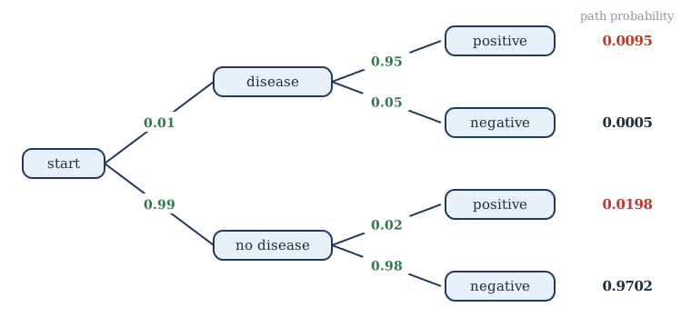
A process that happens in stages is drawn as a tree diagram: each branch carries the conditional probability of that step given the steps before it. The probability of a path is the product of the probabilities along it (the multiplication rule), and the probability of an event is the sum over the paths that lead to it.
That last statement is a theorem.
Theorem 8.2 (the law of total probability)
If \(F_1, \dots, F_n\) are disjoint events with \(F_1 \cup \dots \cup F_n = S\) and each \(p(F_i) > 0\), then for any event \(E\),
Proof. The events \(E \cap F_i\) are disjoint and their union is \(E\), so \(p(E) = \sum_i p(E \cap F_i) = \sum_i p(E \mid F_i)\,p(F_i)\). \(\blacksquare\)
8.4 Bayes' theorem
Conditional probability is not symmetric: \(p(E \mid F)\) and \(p(F \mid E)\) can be very different. The probability that a person is a cricketer given that they play sport is small; the probability that they play sport given that they are a cricketer is 1. Bayes' theorem converts one into the other.
Theorem 8.3 (Bayes' theorem)
If \(p(E) > 0\) and \(0 < p(F) < 1\), then
Proof. By the definition, \(p(F \mid E) = p(E \cap F)/p(E)\). The numerator is \(p(E \mid F)p(F)\) by the multiplication rule, and the denominator is the law of total probability with the partition \(F, \overline{F}\). \(\blacksquare\)
Example 8.6: A medical test
Problem. A disease affects 1% of a population. A test detects the disease in 95% of people who have it, and wrongly gives a positive result for 2% of people who do not. A randomly chosen person tests positive. What is the probability that they have the disease?
Solution. Let \(D\) be "has the disease" and \(T\) be "tests positive". We know \(p(D) = 0.01\), \(p(T \mid D) = 0.95\) and \(p(T \mid \overline{D}) = 0.02\). Figure 8.1 shows the tree. By Bayes' theorem,
Only about one positive result in three is a true positive.
Key idea: base rates
The test is accurate, yet most positives are false, because the disease is rare: the 2% of the large healthy group outnumbers the 95% of the small sick group. Imagine 10,000 people: 100 are sick and 95 of them test positive; 9,900 are healthy and 198 of them test positive. Of the 293 positives, 95 are sick. Forgetting the base rate \(p(D)\) is a common and serious error, sometimes called the base rate fallacy.
Bayes' theorem is the basis of many classifiers. A spam filter estimates, from a collection of messages already sorted, how often each word appears in spam and in genuine mail, and uses Bayes' theorem to turn the words of a new message into a probability that it is spam.
Example 8.7: The Monty Hall problem
Problem. A prize is behind one of three doors, equally likely. You pick door 1. The host, who knows where the prize is, opens one of the other doors that does not hide the prize (choosing at random if both are empty), and offers you the chance to switch to the remaining closed door. Should you switch?
Solution. Switching wins exactly when your first pick was wrong, which has probability \(2/3\): if the prize is behind door 2 or door 3, the host must open the other empty door, and switching takes you to the prize. Sticking wins only if your first pick was right, probability \(1/3\). So switch. The host's choice is not random: it carries information, and that is why the two remaining doors are not equally likely.
8.5 Independence
Definition: independent events
Events \(E\) and \(F\) are independent if \(p(E \cap F) = p(E)\,p(F)\). When \(p(F) > 0\) this is the same as \(p(E \mid F) = p(E)\): knowing that \(F\) happened does not change the probability of \(E\).
Separate coin tosses or dice rolls are modelled as independent. Drawing cards without replacement is not: the first card changes the deck.
Example 8.8: Independent or not?
Problem. A card is drawn from a standard deck. Let \(E\) be "it is a heart", \(F\) be "it is a king" and \(G\) be "it is a red face card". Are \(E\) and \(F\) independent? \(E\) and \(G\)?
Solution. \(p(E) = 1/4\), \(p(F) = 1/13\), and \(p(E \cap F) = 1/52 = (1/4)(1/13)\): independent. \(p(G) = 6/52\) and \(p(E \cap G) = 3/52\), but \(p(E)p(G) = 6/208 = 1.5/52\): not independent. Knowing the card is a red face card doubles the chance that it is a heart, to \(1/2\).
Independent is not the same as disjoint
Disjoint events with positive probabilities are never independent: if \(E\) and \(F\) cannot both happen, then knowing \(F\) happened tells you \(E\) did not.
For more than two events, mutual independence requires the product rule for every subcollection: \(p(E_{i_1} \cap \dots \cap E_{i_k}) = p(E_{i_1}) \cdots p(E_{i_k})\). It is not enough that every pair is independent (Exercise 8).
Bernoulli trials and the binomial distribution
A Bernoulli trial is an experiment with two outcomes, success (probability \(p\)) and failure (probability \(q = 1 - p\)). Many repetitions, mutually independent, are a sequence of Bernoulli trials: tosses of a coin, bits sent over a noisy channel, items from a production line.
Theorem 8.4 (the binomial distribution)
The probability of exactly \(k\) successes in \(n\) independent Bernoulli trials, each with success probability \(p\), is
Proof. A particular sequence with \(k\) successes and \(n - k\) failures has probability \(p^k q^{n-k}\) by independence. There are \(\binom{n}{k}\) such sequences (choose the positions of the successes), and they are disjoint events. \(\blacksquare\)
By the binomial theorem, \(\sum_{k=0}^{n} b(k; n, p) = (p + q)^n = 1\), as it must be.
Example 8.9: Binomial probabilities
Problem. (a) A fair coin is tossed 10 times. What is the probability of exactly 3 heads? Of at least 8 heads? (b) Each bit sent over a channel is flipped with probability \(0.01\), independently. What is the probability that an 8-bit byte arrives with no error?
Solution. (a) \(\binom{10}{3}/2^{10} = 120/1024 \approx 0.117\). At least 8: \((\binom{10}{8} + \binom{10}{9} + \binom{10}{10})/1024 = (45 + 10 + 1)/1024 = 56/1024 \approx 0.055\). (b) \(0.99^8 \approx 0.923\).
8.6 Random variables and expectation
Often we care about a number attached to the outcome: the sum of two dice, the number of heads, the running time of an algorithm on a random input.
Definition: random variable
A random variable is a function \(X\) from the sample space to the real numbers. Its distribution is the list of probabilities \(p(X = r)\) for each value \(r\) it takes.
Definition: expected value
The expected value (or expectation, or mean) of a random variable \(X\) on a sample space \(S\) is
The expectation is the long-run average value. For one roll of a fair die, \(E(X) = (1 + 2 + 3 + 4 + 5 + 6)/6 = 3.5\), a value the die never shows.
Example 8.10: A game
Problem. You pay 10 rupees to roll a die. You win 30 rupees for a six, 10 rupees for a five, and nothing otherwise. What is your expected gain?
Solution. Gain \(X\) is \(30 - 10 = 20\) with probability \(1/6\), \(0\) with probability \(1/6\), and \(-10\) with probability \(4/6\). So \(E(X) = (20 + 0 - 40)/6 = -20/6 \approx -3.33\) rupees per game. On average you lose.
Linearity of expectation
The single most useful fact about expectation is that it adds, whether or not the variables are independent.
Theorem 8.5 (linearity of expectation)
For random variables \(X\) and \(Y\) on the same sample space and real numbers \(a\) and \(b\),
In particular \(E(X_1 + \dots + X_n) = E(X_1) + \dots + E(X_n)\).
Proof. \(E(aX + bY) = \sum_s p(s)(aX(s) + bY(s)) = a\sum_s p(s)X(s) + b\sum_s p(s)Y(s)\). \(\blacksquare\)
The expected sum of two dice is \(3.5 + 3.5 = 7\), with no need to list 36 outcomes. Linearity is most powerful together with indicator variables: for an event \(A\), the indicator \(I_A\) is \(1\) if \(A\) happens and \(0\) otherwise, and \(E(I_A) = p(A)\). To find the expected number of times something happens, write the count as a sum of indicators.
Example 8.11: Expected number of heads, and of fixed points
Problem. (a) What is the expected number of successes in \(n\) Bernoulli trials with success probability \(p\)? (b) \(n\) coats are returned at random to their \(n\) owners. What is the expected number of people who get their own coat?
Solution. (a) Let \(X_i\) indicate success on trial \(i\). Then the number of successes is \(X_1 + \dots + X_n\), and \(E = np\). (Computing \(\sum_k k\binom{n}{k}p^kq^{n-k}\) directly gives the same answer, with much more work.)
(b) Let \(X_i\) indicate that person \(i\) gets their own coat. Then \(E(X_i) = 1/n\), since person \(i\)'s coat is equally likely to be any of the \(n\) coats. So the expected number is \(n \cdot (1/n) = 1\), for every \(n\). The \(X_i\) are not independent, but linearity does not care.
Example 8.12: Waiting for a success
Problem. Bernoulli trials with success probability \(p > 0\) are repeated until the first success. What is the expected number of trials?
Solution. The number of trials \(X\) is \(k\) when the first \(k - 1\) trials fail and the \(k\)-th succeeds: \(p(X = k) = q^{k-1}p\), the geometric distribution. Let \(m = E(X)\). Condition on the first trial: with probability \(p\) it succeeds and \(X = 1\); with probability \(q\) it fails, and then we start afresh having used one trial, so the expected total is \(1 + m\). Hence \(m = p \cdot 1 + q(1 + m)\), so \(m - qm = p + q = 1\), \(pm = 1\) and \(m = 1/p\). On average a die must be rolled 6 times to see a six.
Variance
The expectation says where a random variable is centred; the variance says how widely it spreads.
Definition: variance
The variance of \(X\) is \(V(X) = E\bigl((X - E(X))^2\bigr)\), and its standard deviation is \(\sigma(X) = \sqrt{V(X)}\). Expanding the square gives the formula used in practice: \(V(X) = E(X^2) - E(X)^2\).
For a fair die, \(E(X^2) = (1 + 4 + 9 + 16 + 25 + 36)/6 = 91/6\), so \(V(X) = 91/6 - (7/2)^2 = 35/12 \approx 2.92\). Random variables \(X\) and \(Y\) are independent if \(p(X = r \wedge Y = s) = p(X = r)\,p(Y = s)\) for all \(r, s\); for independent variables, variances add: \(V(X + Y) = V(X) + V(Y)\). So the number of successes in \(n\) Bernoulli trials has variance \(npq\) (each trial contributes \(E(X_i^2) - E(X_i)^2 = p - p^2 = pq\)).
Variance controls how far a random variable is likely to stray from its mean.
Theorem 8.6 (Chebyshev's inequality)
For a random variable \(X\) and any \(r > 0\), \(\;p\bigl(\lvert X - E(X) \rvert \ge r\bigr) \le V(X)/r^2\).
Proof. Let \(A\) be the event \(\lvert X - E(X) \rvert \ge r\). Then \(V(X) = \sum_s p(s)(X(s) - E(X))^2 \ge \sum_{s \in A} p(s)(X(s) - E(X))^2 \ge \sum_{s \in A} p(s)\,r^2 = r^2 p(A)\). \(\blacksquare\)
For 10,000 tosses of a fair coin, the number of heads has mean 5000 and variance 2500, so the probability of being 500 or more away from 5000 is at most \(2500/500^2 = 0.01\). This is a first version of the law of large numbers: the proportion of heads settles down near \(1/2\).
8.7 Summary
Summary
- With equally likely outcomes, \(p(E) = \lvert E \rvert/\lvert S \rvert\): probability is counting. In general a distribution assigns probabilities that sum to 1.
- \(p(\overline{E}) = 1 - p(E)\) and \(p(E \cup F) = p(E) + p(F) - p(E \cap F)\). Use complements for "at least one".
- \(p(E \mid F) = p(E \cap F)/p(F)\). Multiply along the branches of a tree; add over the paths to an event (total probability).
- Bayes' theorem reverses a conditional probability; never forget the base rate.
- \(E\) and \(F\) are independent when \(p(E \cap F) = p(E)p(F)\). \(n\) independent trials give the binomial distribution \(\binom{n}{k}p^kq^{n-k}\).
- \(E(X) = \sum r\,p(X = r)\). Linearity of expectation holds without independence; with indicator variables it gives \(np\) for the binomial, 1 for fixed points of a random permutation, and \(1/p\) for the geometric waiting time.
- \(V(X) = E(X^2) - E(X)^2\); Chebyshev's inequality bounds the chance of large deviations.
8.8 Exercises
Exercise 1
Two dice are rolled. Find the probability that (a) the sum is at least 10, (b) the two numbers differ by exactly 2.
Answer
(a) Sums 10, 11, 12 occur in \(3 + 2 + 1 = 6\) of 36 outcomes: \(1/6\). (b) Pairs \((1,3), (2,4), (3,5), (4,6)\) and their reverses: \(8/36 = 2/9\).
Exercise 2
A bit string of length 8 is chosen at random. What is the probability that it contains at least one 0? Exactly four 1s?
Answer
At least one 0: \(1 - 1/256 = 255/256\). Exactly four 1s: \(\binom{8}{4}/256 = 70/256 = 35/128\).
Exercise 3
A box contains 5 red and 3 blue balls. Two are drawn without replacement. Find the probability that they are the same colour.
Answer
Both red: \(\frac{5}{8}\cdot\frac{4}{7} = \frac{20}{56}\). Both blue: \(\frac{3}{8}\cdot\frac{2}{7} = \frac{6}{56}\). Total \(26/56 = 13/28\).
Exercise 4
In Example 8.6, suppose the person takes a second, independent test of the same kind, and it is also positive. What is now the probability that they have the disease?
Answer
Use the answer to the first test as the new prior, \(0.0095/0.0293 \approx 0.3242\). Then \(p(D \mid \text{both}) = \dfrac{0.95 \times 0.3242}{0.95 \times 0.3242 + 0.02 \times 0.6758} \approx \dfrac{0.3080}{0.3215} \approx 0.958\). Two positives make the disease very likely.
Exercise 5
A fair coin is tossed 6 times. What is the probability of more heads than tails?
Answer
4, 5 or 6 heads: \((\binom{6}{4} + \binom{6}{5} + \binom{6}{6})/64 = (15 + 6 + 1)/64 = 22/64 = 11/32\).
Exercise 6
A student guesses every answer on a test of 20 questions, each with 4 options. What is the expected number of correct answers, and the variance?
Answer
Binomial with \(n = 20\), \(p = 1/4\): expectation \(5\), variance \(npq = 20 \cdot \frac14 \cdot \frac34 = 3.75\).
Exercise 7
A random permutation of \(1, 2, \dots, n\) is chosen. What is the expected number of positions \(i\) (with \(1 \le i < n\)) at which the entry in position \(i + 1\) is larger than the entry in position \(i\)?
Answer
For each \(i\) let \(X_i\) indicate an ascent at \(i\). The two entries in positions \(i\) and \(i + 1\) are equally likely to be in either order, so \(E(X_i) = 1/2\). By linearity the expected number of ascents is \((n - 1)/2\).
Exercise 8
Two fair coins are tossed. Let \(A\) be "the first is heads", \(B\) be "the second is heads" and \(C\) be "the two coins match". Show that each pair of \(A, B, C\) is independent, but the three are not mutually independent.
Answer
Each event has probability \(1/2\), and each pairwise intersection is \(\{HH\}\), of probability \(1/4 = \frac12 \cdot \frac12\). But \(p(A \cap B \cap C) = p(\{HH\}) = 1/4 \ne 1/8 = p(A)p(B)p(C)\). (Knowing \(A\) and \(B\) determines \(C\).)
Exercise 9
How many rolls of a pair of dice are needed, on average, to get a double six?
Answer
Geometric with \(p = 1/36\): an expected 36 rolls.
8.9 Quiz
Check your understanding of discrete probability
Exercise 1
Two dice are rolled. The probability that the sum is 7 is
- 1/11
- 1/6
- 1/12
- 7/36
Answer
1/6
Exercise 2
In a group of 23 people the probability that two share a birthday is about
- 0.06
- 0.23
- 0.51
- 0.97
Answer
0.51
Exercise 3
Disjoint events with positive probability are
- always independent
- never independent
- sometimes independent
Answer
never independent
Exercise 4
What is the expected value of one roll of a fair six-sided die? (decimal)
Answer
3.5
Exercise 5
Linearity of expectation E(X + Y) = E(X) + E(Y) requires X and Y to be
- independent
- disjoint
- identically distributed
- nothing: it always holds
Answer
nothing: it always holds
Exercise 6
On average, how many tosses of a fair coin are needed to get the first head?
Answer
2
Exercise 7
A rare disease and an accurate test give a positive result. The probability of disease is low mainly because of
- the base rate
- the test's sensitivity
- independence
- Chebyshev's inequality
Answer
the base rate