Classical Orbital Elements and Coordinate Transformations
This appendix provides the complete mathematical reference for classical orbital mechanics, coordinate frames, and the transformations used throughout the book. All derivations follow the conventions of Bate, Mueller, and White (1971) and Vallado (2013).
Standard Gravitational Parameters
The standard gravitational parameter \(\mu = GM\) combines the universal gravitational constant \(G = 6.674\,30 \times 10^{-11}\) m\(^3\) kg\(^{-1}\) s\(^{-2}\) with the mass \(M\) of the central body. Using \(\mu\) rather than \(G\) and \(M\) separately eliminates the relative uncertainty in \(G\) from precision orbit determination.
| Body | \(\mu\) (km\(^3\) s\(^{-2}\)) | \(\mu\) (m\(^3\) s\(^{-2}\)) | Source |
|---|---|---|---|
| Sun | \(1.327\,124\,400\,18 \times 10^{11}\) | \(1.327\,124\,400\,18 \times 10^{20}\) | IAU 2012 |
| Earth | \(3.986\,004\,418 \times 10^{5}\) | \(3.986\,004\,418 \times 10^{14}\) | EGM2008 |
| Moon | \(4.902\,800\,066 \times 10^{3}\) | \(4.902\,800\,066 \times 10^{12}\) | DE430 |
| Mars | \(4.282\,837\,59 \times 10^{4}\) | \(4.282\,837\,59 \times 10^{13}\) | MRO/MGS |
| Jupiter | \(1.266\,865\,349 \times 10^{8}\) | \(1.266\,865\,349 \times 10^{17}\) | Juno |
| Saturn | \(3.793\,120\,62 \times 10^{7}\) | \(3.793\,120\,62 \times 10^{16}\) | Cassini |
| Venus | \(3.248\,585\,92 \times 10^{5}\) | \(3.248\,585\,92 \times 10^{14}\) | MESSENGER |
| Mercury | \(2.203\,186\,86 \times 10^{4}\) | \(2.203\,186\,86 \times 10^{13}\) | MESSENGER |
Earth Physical Constants
Table 2 lists the primary physical constants of the Earth used in satellite orbit computation, attitude determination, and communications link analyses.
| Constant | Symbol | Value | Units |
|---|---|---|---|
| Equatorial radius | \(R_E\) | 6 378.137 0 | km |
| Polar radius | \(R_p\) | 6 356.752 3 | km |
| Flattening | \(f\) | 1/298.257 223 563 | – |
| Mean radius | \(\bar{R}_E\) | 6 371.008 8 | km |
| Grav. parameter | \(\mu_E\) | 398 600.441 8 | km\(^3\) s\(^{-2}\) |
| \(J_2\) zonal harmonic | \(J_2\) | \(1.082\,626\,68 \times 10^{-3}\) | – |
| \(J_3\) zonal harmonic | \(J_3\) | \(-2.532\,435 \times 10^{-6}\) | – |
| \(J_4\) zonal harmonic | \(J_4\) | \(-1.619\,331 \times 10^{-6}\) | – |
| \(J_5\) zonal harmonic | \(J_5\) | \(-2.277\,161 \times 10^{-7}\) | – |
| Earth rotation rate | \(\omega_E\) | \(7.292\,115\,0 \times 10^{-5}\) | rad s\(^{-1}\) |
| Speed of light (vacuum) | \(c\) | 299 792 458 | m s\(^{-1}\) |
| Standard gravity | \(g_0\) | 9.806 65 | m s\(^{-2}\) |
| Solar pressure constant | \(P_\odot\) | \(4.560 \times 10^{-6}\) | N m\(^{-2}\) |
| Sidereal day | \(T_\text{sid}\) | 86 164.090 5 | s |
| Solar day | \(T_\odot\) | 86 400.000 0 | s |
The Six Classical Orbital Elements
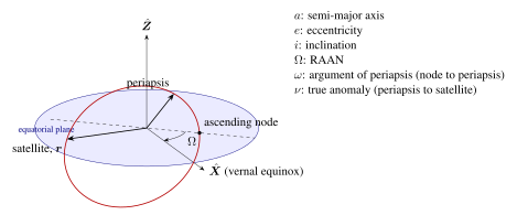
Any two-body Keplerian orbit is uniquely determined by six scalar constants—the Classical Orbital Elements (COE), also called Keplerian elements. Three elements define the shape and size of the ellipse; three orient that ellipse in inertial space.
Size and Shape
- \(a\) – Semi-major axis (km).
- Half the longest diameter of the orbital ellipse. It sets the orbital energy \(\mathcal{E} = -\mu/(2a)\) and the period \(T = 2\pi\sqrt{a^3/\mu}\).
- \(e\) – Eccentricity (dimensionless).
- Measures the deviation from a circle. Ranges from \(0\) (circular) through \(<1\) (elliptical) to \(1\) (parabolic) and \(>1\) (hyperbolic). Related to the semi-latus rectum by \(p = a(1-e^2)\).
- \(\nu\) – True anomaly (rad or deg).
- Angle measured in the orbital plane from the perigee direction to the satellite, in the direction of motion. It is the position element; all five others are constants of integration.
Orientation in Inertial Space
- \(i\) – Inclination (rad or deg).
- Angle between the orbital plane and the equatorial plane, measured at the ascending node. \(0 \le i \le \pi\). Prograde orbits have \(i < 90\degree{}\); retrograde have \(i > 90\degree{}\).
- \(\Omega\) – Right Ascension of the Ascending Node (RAAN) (rad or deg).
- Angle in the equatorial plane from the vernal equinox direction (\(\hat{\boldsymbol{X}}\)) eastward to the ascending node. Ranges from 0 to \(2\pi\).
- \(\omega\) – Argument of Perigee (AoP) (rad or deg).
- Angle in the orbital plane from the ascending node to perigee, measured in the direction of motion. Undefined for circular orbits (\(e=0\)).
Anomaly Conversions
True Anomaly to Eccentric Anomaly
The eccentric anomaly \(E\) is an auxiliary angle defined on a circumscribed circle of radius \(a\). The conversion is:
Careful use of the atan2 function is required to resolve the quadrant ambiguity: \(E\) and \(\nu\) always lie in the same half-plane (\(0 \le \nu < \pi \Leftrightarrow 0 \le E < \pi\)).
Eccentric Anomaly to Mean Anomaly (Kepler’s Equation)
The mean anomaly \(M\) grows linearly in time:
where \(n = \sqrt{\mu/a^3}\) is the mean motion and \(t_p\) is the time of perigee passage.
Mean Anomaly to Eccentric Anomaly: Newton–Raphson Solution
Kepler’s equation (2) cannot be inverted analytically; numerical methods are required. The Newton–Raphson iteration is:
Algorithm A.1 – Kepler Equation Solver
-
Set \(E_0 = M\) for \(e < 0.8\), or \(E_0 = \pi\) for \(e \ge 0.8\).
-
Iterate (3) until \(|E_{k+1} - E_k| < 10^{-12}\) rad (typically 3–6 iterations for \(e < 0.97\)).
-
Return \(E\) modulo \(2\pi\).
For near-parabolic orbits (\(e > 0.999\)) the Battin (1987) universal variable formulation is recommended.
Position and Velocity in the Perifocal Frame
The perifocal (PQW) frame has unit vectors: \(\hat{\boldsymbol{p}}\) pointing toward perigee, \(\hat{\boldsymbol{q}}\) in the orbital plane \(90\degree{}\) ahead of perigee (in the direction of motion), and \(\hat{\boldsymbol{w}} = \hat{\boldsymbol{p}}\times\hat{\boldsymbol{q}}\) normal to the orbital plane.
where the semi-latus rectum \(p = a(1-e^2)\).
Rotation Matrices and ECI State Vector
Elementary Rotation Matrices
Positive rotations follow the right-hand rule about axis \(k\):
Perifocal to ECI Transformation
The ECI position vector is obtained by three successive rotations that undo the three orientation angles:
Writing out the composite direction cosine matrix \(\boldsymbol{Q} = \boldsymbol{R}_3(-\Omega)\,\boldsymbol{R}_1(-i)\,\boldsymbol{R}_3(-\omega)\):
The same rotation applies to velocity: \(\boldsymbol{v}_{\text{ECI}} = \boldsymbol{Q}\,\boldsymbol{v}_{\text{peri}}\).
State Vector to Orbital Elements (Inverse Problem)
Given position \(\boldsymbol{r}_{\text{ECI}}\) and velocity \(\boldsymbol{v}_{\text{ECI}}\) in ECI coordinates, the classical elements follow from:
Algorithm A.2 – State Vector to Classical Orbital Elements
-
Compute specific angular momentum: \(\boldsymbol{h} = \boldsymbol{r} \times \boldsymbol{v}\), \(h = |\boldsymbol{h}|\).
-
Compute node vector: \(\boldsymbol{N} = \hat{\boldsymbol{K}} \times \boldsymbol{h}\), \(N = |\boldsymbol{N}|\).
-
Compute eccentricity vector: \(\boldsymbol{e}_v = \dfrac{1}{\mu}\!\left[ \left(v^2 - \dfrac{\mu}{r}\right)\boldsymbol{r} - (\boldsymbol{r}\cdot\boldsymbol{v})\boldsymbol{v} \right]\), \(e = |\boldsymbol{e}_v|\).
-
Compute specific mechanical energy: \(\mathcal{E} = v^2/2 - \mu/r\).
-
Semi-major axis: \(a = -\mu/(2\mathcal{E})\).
-
Inclination: \(i = \arccos(h_z/h)\).
-
RAAN: \(\Omega = \arccos(N_x/N)\). If \(N_y < 0\), then \(\Omega = 2\pi - \Omega\).
-
Argument of perigee: \(\omega = \arccos(\boldsymbol{N}\cdot\boldsymbol{e}_v/(Ne))\). If \(e_{v,z} < 0\), then \(\omega = 2\pi - \omega\).
-
True anomaly: \(\nu = \arccos(\boldsymbol{e}_v\cdot\boldsymbol{r}/(er))\). If \(\boldsymbol{r}\cdot\boldsymbol{v} < 0\), then \(\nu = 2\pi - \nu\).
Special cases: circular orbits (\(e < 10^{-4}\)) use the argument of latitude \(u = \omega + \nu\); equatorial orbits (\(i < 0.001\degree{}\)) use the true longitude of perigee \(\tilde{\omega} = \Omega + \omega\).
ECI to ECEF Transformation
The Earth-Centred Earth-Fixed (ECEF) frame rotates with the Earth. The transformation from ECI to ECEF requires accounting for Earth rotation, precession, nutation, and polar motion. For satellite orbit prediction to \(<1\) km accuracy the following simplified form is sufficient:
Greenwich Apparent Sidereal Time (GAST)
GAST at epoch \(t\) (Julian date \(J\)) is computed as follows. Define the Julian centuries from J2000.0:
Earth Rotation Angle (ERA):
where \(D_u = J - 2\,451\,545.0\) is the number of UT1 days from J2000.0. Adding the equation of the equinoxes \(\Delta\psi\cos\varepsilon\) gives GAST. For most engineering applications, Greenwich Mean Sidereal Time (GMST) is adequate:
ECEF to Geodetic Coordinates
Given ECEF position \((X, Y, Z)\), geodetic longitude \(\lambda\), latitude \(\phi\), and altitude \(h\) are found as follows.
Geodetic latitude and altitude require iteration because the Earth is an oblate spheroid. Define:
Bowring’s Iterative Method:
-
Initial estimate: \(\phi_0 = \mathrm{atan2}(Z, p(1-e_E^2))\).
-
Compute radius of curvature in prime vertical: \(N = R_E / \sqrt{1 - e_E^2 \sin^2\phi}\).
-
Update: \(\phi = \mathrm{atan2}\!\left(Z + e_E^2 N\sin\phi,\; p\right)\).
-
Repeat steps 2–3 until \(|\Delta\phi| < 10^{-11}\) rad (3 iterations converge to sub-millimetre accuracy).
-
Altitude: \(h = p/\cos\phi - N\). At poles (\(\phi = \pm 90\degree{}\)): \(h = |Z|/\sin\phi - N(1-e_E^2)\).
Two-Line Element Set (TLE) Format
The TLE format, standardised by USSTRATCOM/Space-Track, encodes a near-earth satellite state compatible with the SGP4/SDP4 propagators.
| Col. | Field | Example | Description |
|---|---|---|---|
| 1 | Line number | 1 |
Always 1 |
| 3–7 | Satellite number | 25544 |
NORAD catalogue ID |
| 8 | Classification | U |
U=Unclassified, C=Classified |
| 10–11 | Int. desig. year | 98 |
Launch year (2-digit) |
| 12–14 | Int. desig. launch | 067 |
Launch number in year |
| 15–17 | Int. desig. piece | A |
Piece of launch |
| 19–20 | Epoch year | 24 |
Year (2-digit) |
| 21–32 | Epoch day | 264.51782528 |
Day of year (fractional) |
| 34–43 | Ballistic coeff. | .00001764 |
First deriv. of mean motion/2 (rev/day\(^2\)) |
| 45–52 | 2nd deriv. mean mo. | 00000+0 |
Second deriv./6 (rev/day\(^3\)) |
| 54–61 | BSTAR drag term | 31088-3 |
SGP4 drag coefficient (1/R\(_E\)) |
| 63 | Element set type | 0 |
0 = distributed to public |
| 65–68 | Element set no. | 999 |
Incrementing integer |
| 69 | Checksum | 3 |
Modulo-10 checksum |
| Col. | Field | Example | Description |
|---|---|---|---|
| 1 | Line number | 2 |
Always 2 |
| 3–7 | Satellite number | 25544 |
Same as Line 1 |
| 9–16 | Inclination | 051.6400 |
Degrees |
| 18–25 | RAAN | 254.6611 |
Degrees |
| 27–33 | Eccentricity | 0001764 |
Decimal point assumed at start |
| 35–42 | Arg. of perigee | 148.9962 |
Degrees |
| 44–51 | Mean anomaly | 211.2021 |
Degrees |
| 53–63 | Mean motion | 15.49560679 |
Revolutions per day |
| 64–68 | Rev. at epoch | 56353 |
Revolution number |
| 69 | Checksum | 7 |
Modulo-10 checksum |
TLE Epoch Convention
The TLE epoch day is the fractional day of year in UTC. To convert to a Julian date:
where \(J_{\text{Jan 0.0}}\) is the Julian date of 0 January of the epoch year (equivalently, 31 December of the previous year at 00:00:00 UTC).
Mean Motion and Semi-major Axis
The TLE mean motion \(n_0\) (rev/day) relates to the osculating semi-major axis via the SGP4 Kozai-mean element definition, not a simple Keplerian relation. The approximate Keplerian relation is:
Checksum Calculation
Each TLE line ends with a modulo-10 checksum. Sum the integer value of each digit character; treat each minus sign as 1, spaces and letters as 0. Take the result modulo 10.
Common Orbit Types: Reference Elements
Table 5 lists nominal orbital elements for representative satellites. All values are approximate; use current TLEs for operational calculations.
| Satellite / Type | \(a\) | \(e\) | \(i\) | \(\Omega\) | \(\omega\) | \(n\) | Period |
| (km) | (deg) | (deg) | (deg) | (rev/d) | |||
| ISS (LEO) | 6 797 | 0.0004 | 51.64 | – | – | 15.49 | 93.0 min |
| Starlink (550 km shell) | 6 921 | 0.0001 | 53.0 | – | – | 15.08 | 95.5 min |
| Envisat (SSO) | 7 159 | 0.0001 | 98.55 | – | – | 14.33 | 100.5 min |
| GPS Block IIF | 26 560 | 0.0001 | 55.0 | – | – | 2.006 | 11.97 h |
| GLONASS-M | 25 508 | 0.001 | 64.8 | – | – | 2.131 | 11.26 h |
| Galileo FOC | 29 600 | 0.0003 | 56.0 | – | – | 1.705 | 14.08 h |
| Molniya (HEO) | 26 556 | 0.72 | 63.4 | – | 270.0 | 2.006 | 11.97 h |
| GOES-16 (GEO) | 42 164 | \(<0.001\) | \(<0.1\) | – | – | 1.003 | 23.93 h |
| Meteosat-12 (GEO) | 42 164 | \(<0.001\) | \(<0.1\) | – | – | 1.003 | 23.93 h |
| \(a\) = semi-major axis from Earth’s centre; \(n\) = mean motion; – = varies by orbital plane. | |||||||